Diffusion of Polymer Chains

A small particle diffuses in solution and melt due to fluctuations of the number of nearby molecules randomly colliding with the particle from different directions. Polymer molecules are typically much larger than solvent molecules (or monomers) but still small enough that random collisons with other molecules noticeably move the polymer. The net transport of molecules due to diffusion is typically caused by a concentration or pressure gradient. According to Fick's first law of diffusiion¹, the diffusive flux j_i (i.e. the amount of substance i diffusing through a unit area per unit time) due to a concentration gradient is proportional to the concentration gradient:

j_i = -D_i ∇c_i

If the concentration varies only in one direction, Ficks first law reduces to

j_i,x = -D_i δc_i /δx

where D_i is called the diffusion coefficient of substance i and c_i is its concentration at x. The rate of change of concentration is given by Fick's second law of diffusion:

δc_i /δt = -δj_i,x /δx = D_i δ²c_i /δx²

And if the concentration depends on all three coordinates,

δc_i /δt  = D_i ∇²c_i

This is the so-called diffusion equation.
The random motion of a particle (i.e. its trajectory) resembles a random conformation of a Gaussian polymer chain. In other words, a random motion of a particle describes an ideal polymer chain.

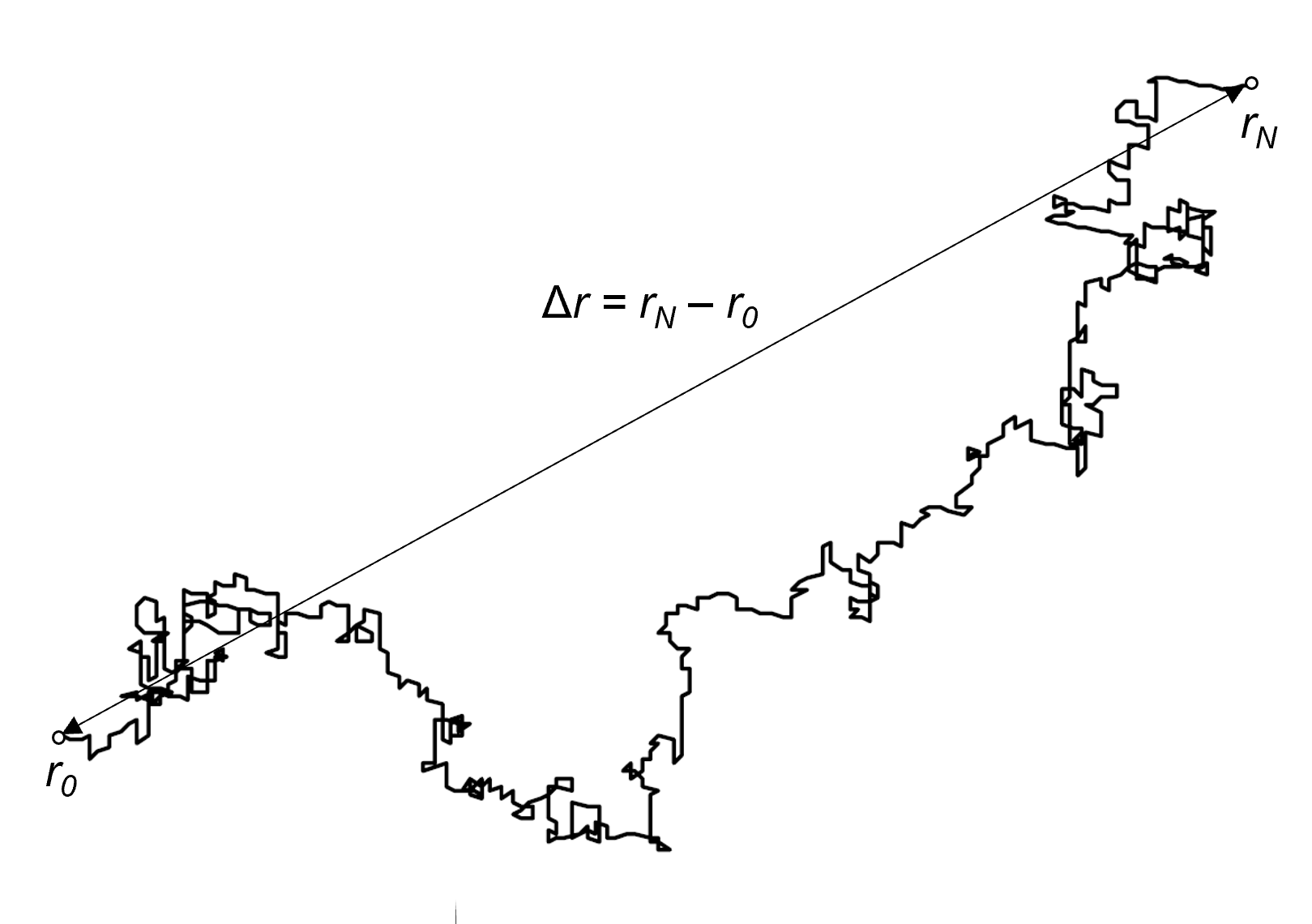
Then the mean square displacement of a N step walk in time t = N t₁ is equivalent to the mean-square end-to-end distance ⟨R²⟩ of an ideal polymer chain:

⟨(r_N - r₀)²⟩ ≅ 〈[r(t) - r(0)²]⟩

The average displacement of a particles in time t is (6Dt)^½ whereas the average root-mean-square end-to-end distance of an ideal polymer chain is lN^½. Then the Diffusion coefficient is given by

D = ⟨(r_N - r₀)²⟩ / 6t = Nl² / (6N t₁) = l² / 6t₁

A Gaussian chain has the probability distribution

P(r_N, r₀, N) = (2 πNl²/ 3)^-3/2 exp[-3(r_N - r₀)² / (2Nl²)]

Which now can be written as²

P[r(t), r(0), t] = (4 πDt)^-3/2 exp{-[r(t) - r(0)]² / (4Dt)}

and in one dimension:

P[x(t), x(0), t] = (4 πDt)^-1/2 exp[-([x(t) - x(0)]² / (4Dt)]

The figure below shows the probability distribution of a diffusing particle for a one dimensional random walk. The curves are given as a function of [x(t) - x(0)]/l for = 0.1, 0.25, 1, and 10, where l is the unit length. At t = 0, the particle is at x(0). Then P[x(t₁), x(0), t₁] is the probability that the particle will reach the point x(t₁) at time t₁.

 

Probability distribution of a Gaussian Particle

The dynamic of an ideal (Gaussian) polymer chain was first investigated by Rouse in 1953.³ He showed that the motion of a polymer chain in its melt state and in solution can be described with a simple bead-spring model. In this model, the chain is composed of a series of beads and springs. Each spring has a length of l and a spring constant of 3kT/l². The calculations are rather involved but the results are remarkably simple. According to the Rouse model, the mean square displacement of the center of mass R_g in time t is directly proportional to the time:

〈[R_g(t) - R_g(0)]²⟩ = (6kT / Nζ) · t

where ζ is the friction coefficient of a bead. Using the Einstein relation D = kT / ζ , the diffusion coefficient of the center of mass can be written as

D_coil = kT / Nζ

Thus the diffusion coeffient decreases inversely with the chain length N (number of beads).

The time correlation of the end-to-end distance of a polymer coil decays like²

〈R(t) R(0)〉 = (8Nl²/ π²) ∑_p=1,3,5... p^-2 exp(-tp²/τ₁) ≈ (8/π²) 〈R²〉 exp(-t/τ₁)

where τ₁ is the relaxation time of mode p = 1, which is often called the maximum relaxation time of the polymer coil:^2,4

τ₁ = N²l²ζ / (3π²kT) ≈ Nl² / D_coil ≈ ⟨R²〉 / D_coil

The relaxation time τ₁ is typically very short. Thus a polymer chain loses its memory very quickly (exponentially) with a characteristic time τ₁. Furthermore, a polymer diffuses a distance of the order of its coil size during the Rouse time τ₁:

⟨R²〉^1/2 = 〈[r(t) - r(0)²]〉^1/2 ≈ (D_coil τ₁)^1/2

Rubinstein and Colby³ suggested that the relationship τ₁  ≈ ⟨R²〉 / D_coil is universal, i.e. it should also apply to real chains of size R = l N^ν. Then the relaxation time τ follows the scaling relationship

τ₁ ≈ ⟨R²〉 / D_coil = l²N^2νN ζ / kT = N^2ν+1τ₀

where τ₀ = ζ l²/ kT is the relaxation time of an individual bead. For time scales shorter than τ₀ the polymer behaves like an elastic body. In other words, this time is too short for the polymer to disentangle and to dissipate mechanical energy as heat. If, on the other hand, τ₀ < t < τ₁, the polymer shows viscoelastic behavior and for very large time scales, t >> τ₁, the polymer behaves like an ordinary liquid.

It has been demonstrated experimentally that τ₁ of a polymer in a θ-solvent is proportional to N^3/2 and not N². This discrepancy is due to hydrodynamic interactions⁷ which are not accounted for within Rouse's model. Another model was developed by Zimm⁵ which correctly predicts τ₁≅ N^3/2. Zimm assumed that the moving polymer coil drags some of the surrounding solvent molecules with it which increases the friction coefficient ζ. In the case of a non-draining polymer coil, a polymer behaves like a solid particle and Stokes law applies, thus⁶

ζ_p ≈ η_s R ≈ η_s lN^ν

where η_s is the viscosity of the surrounding solvent. Using the Einstein relation D = kT / ζ , the diffusion coefficient of the center of mass can be written as

D_coil ≈ kT / η_s lN^ν

Zimm's exact calculation for an ideal chain reads⁵

D_coil = 0.192 kT / η_s lN^ν

Zimm's relaxation time τ is of order

τ₁ ≈ ⟨R²〉 / D_coil ≈ η_sR³/kT ≈ η_sl³N^3ν/kT ≈ N^3ντ₀

which is the time a particle diffuses a distance of the order of its size. The Zimm model is in good agreement with the experimentally observed behavior of a polymer in a dilute solution:

D_coil ∝ M^ν;   τ₁ ∝ M^3ν

References & Notes

1. Adolf Fick, Annalen der Physik, 170, 59-86 (1855)

2. Masao Doi, Introduction to Polymer Physics, New York 1997

3. P. E. Rouse, J. Chem. Phys. 21, 7, 1272-1280 (1953)

4. Michael Rubinstein and Raph Colby, Polymer Physics, 1st Ed., New York 2003

5. B. H. Zimm, Journal of Chemical Physics, 24, 269-278 (1956)

6. Stokes law for a spherical particels of radius R reads ζ ≈ 6π ηR. However, polymers are not spherical. Thus, the numerical prefactor will be be different.