Thermogravimetric Analysis
of Polymers
Thermogravimetric analysis (TGA) is one of the most popular
analysis techniques to study the decomposition process of polymeric
materials in controlled atmospheres at various temperatures.
Thermal degradation usually produces volatile compounds. Thus, measuring the weight loss at different temperatures provides information about the thermal stability of polymeric
materials.
The onset of weight loss is often used to define the upper temperature limit of thermal stability. However, in
many cases degradation has already taken place without a detectable weight loss, for example by chain scission or cross-linking reactions. Thus, in some cases the upper service temperature is noticeably lower than the onset of weight loss. Nevertheless, thermogravimetric methods are often an excellent choice to study thermal degradation processes of polymers.
Both isothermal and dynamic thermogravimetric methods are employed. In the case of
a dynamic TGA, the weight loss of a sample is recorded while the temperature is continuously increased at a constant rate
in a controlled atmosphere whereas an isothermogravimetric analysis (IGA) meausures the
weight loss at a constant temperature as a function of time and
atmosphere.
For a reaction of the type
A(solid) → B(solid) + C(gas)
the rate of weight loss, i.e. the amount of gas released will depend on the heating rate and temperature and can be described with an empirical equation of the form:
Rd = dα/ dt = k(T) · f(α)
where k is the rate constant of the decomposition process, f(α) an (empirical) reaction model and α is the extend of conversion which is defined as
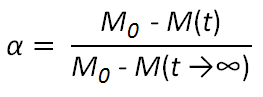
where M0 is the initial weight and M(t) the weight at time t.
A popular equation to describe the decomposition kinetic is1,3
f(α) = c · αm · (1 - α)n · [- ln(1 - α)]p
with m, n, and p parameters that depend on the reaction mechanism. They are usually determined by model fitting.
| Mechanism1,7-8 | f(α) | g(α) |
| Power Law 1 | 4α3/4 | α1/4 |
| Power Law 2 | 3α2/3 | α1/3 |
| Power Law 3 | 2α1/2 | α1/2 |
| First Order | (1-α) | -ln(1-α) |
| Second Order | (1-α)2 | (1-α)-1 - 1 |
| Third Order | (1-α)3 | [(1-α)-2 - 1] / 2 |
| Diffusion 1-D | 1/2α-1 | α2 |
| Diffusion 2-D | [-ln(1-α)]-1 | (1-α) ln(1-α) + α |
| Diffusion 3-D | [1-(1-α)1/3]2 | |
| Contracting Area | 2(1-α)1/2 | 1 - (1-α)1/2 |
| Contracting Volume | 3(1-α)2/3 | 1 - (1-α)1/3 |
| Avarami-Erofeev (A2) | 2(1-α)[-ln(1-α)]1/2 | [-ln(1-α)]1/2 |
| Avarami-Erofeev (A3) | 3(1-α)[-ln(1-α)]2/3 | [-ln(1-α)]1/3 |
| Avarami-Erofeev (A4) | 4(1-α)[-ln(1-α)]3/4 | [-ln(1-α)]1/4 |
The rate constant k describes the relationship between the reaction rate (dα/dt) and the extend of conversion α. Its temperature dependence can be described with an Arrhenius equation:
k(T) = A · exp(- Ea / RT)
where R is the gas constant and T the temperature. The two parameters Ea and A are the activation energy and the frequency factor of the reaction. Combining the equation of k(T) and Rd gives
dα/dt = k(T) · f(α) = A · exp(- Ea / RT) · f(α)
Integration of the expression dα/ dt = k(T) · f(α),
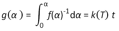
and substitution for k(T) yields after rearranging
g(α)/t = A · exp(- Ea / RT)
This expression is often written in its logarithmic form
ln t = ln[g(α) / A] - (Ea / RT)
Choosing a fixed value of α, the first term on the right hand side of this equation is a constant. Then apparent activation energy, Ea, can be determined from the slope of a log t against T-1 plot.
The equation above can also be expressed as a function of heating rate β = dT/dt:
β · dα / dT = A · exp(- Ea / RT) · f(α)
ln(β dα / dT)= ln [A / f(α)] - Ea / RT
Thus measuring the temperature, T, and the conversion rate dα / dT for a fixed extend of conversion α at different heating rates β and plotting ln(β dα / dT) versus 1/T yields the activation energy Ea. This isoconversional method has been suggested by Friedman.2
Many other approximate equations for the calculation of the apparent activation energy have been suggested. Two of the most popular methods are:
Flynn-Wall-Ozawa4,5
ln β = ln [AEa / g(α)R] - 5.331 - 1.052 Ea / RT
Coats-Redfern6
ln [g(α) / T2] = ln
[AR / βEa] - Ea / RT
Both methods are based on using approximations for the expression
![]()
The accuracy of these methods depends on the extend of conversion α. Usually conversions between 2% to 20% give results of reasonable accuracy.
The effective activation energy of thermal-oxidative degradation is often a good indicator for the heat stability of a plastics. However, the activation energy is not always a constant but often depends on the extend of reaction as well as on the atmosphere. In the case of PE and PP, values between about 150 and 250 kJ/mol have been measured under nitrogen whereas polystyrene (PS) has a practically constant activation energy of about 200 kJ/mol.9 The activation energy will also be affected by the degree of branching because tertiary carbon atoms are less stable than secondary carbon atoms. Under air, the activation energy is often much lower. For example, the activation energy of PS is typically in the range of 125 kJ/mol and that of PE and PP in the range of 80 to 90 kJ/mol.9
Notes & References
S. Vyazovkin, C.A. Wight, Rev. Phys. Chem., Vol. 17, 3, 407 - 453 (1998)
-
H. Friedman, J. Poly. Sci., Part C, vol. 6, p. 183 - 195 (1964)
-
The decomposition reaction is often assumed to be of first order, n = 1.
dα/dT = A/β · exp(- Ea/RT) · (1 - α)
This greatly simplifies the calculation:
J.H. Flyn, L.A. Wall, J. Poly. Sci. Part B: Poly. Lett., Vol 4, p 323 - 328 (1966)
-
T. Ozawa, Bull. Chem. Soc. Jpn., Vol 38, p. 1881-6 (1965)
-
A.W. Coats, J.P. Redfern, Nature, Vol. 201, p 68 - 69 (1964)
-
A. Aboulkas, K. El. Harfi, Oil Shale, Vol 25, No.4, p 426-443 (2008)
-
G.C. Vasconceles, R.L. Mazur, B. Ribeiro, E.C. Botelho, M.L. Costa,
Mat. Res. 17(1), 227-235 (2014) -
J.D. Peterson, S. Vyazovkin, and C.A. Wight, Macromol. Chem. Phys., 202, 775-784 (2001)