Compressible Regular Solution Free Energy Model of Mixtures
Part 1

The thermodynamics of (binary) polymer solutions and blends is often described with the classical Flory-Huggins theory^1-3. However, this model has many short-commings; in the Flory-Huggins formalism, the binary interaction parameter, χ_i,j, is assumed to be inversely proportional to temperature and independent of composition and pressure. For most mixtures, this assumption leads to expressions that are unable to describe the full range of phase behavior observed for polymer blends and solutions.⁴ It was found that for most polymer solutions the interaction paramerer, χ_i,j, is a complex function of several independent variables that are often unknown and cannot be easily predicted, i.e., they have to be measured. Furthermore, expressions that describe the correct temperature and concentration dependency of the free energy of mixing are often quite complex and difficult to solve and do not always provide an accurate description of the system's phase behavior. For this reason, it is desirable to express all concentration and temperature dependent parameters as a function of pure component properties. One such model was developed by Ruzette and Mayes (2001)⁵. It predicts the free energy of mixing of compressible polymer blends, and is based on a modification of the regular solution model. This model captures, at least semi-quantitatively, the phase behavior of weakly interacting polymer pairs using only pure component properties such as mass density, solubility parameter, and thermal expansion coefficient, i.e., this model avoids the direct calculation of the temperature and concentration dependency of the interaction parameter.

The regular solution free energy model of Ruzette and Mayes is based on following simple mixing rules:

• The closed packed volume of the mixture is equal to the sum of the pure component closed packed volumes:
  V_hc,mix = r₁ N₁ v_hc,1 + r₂ N₂ v_hc,2 + ...
  where v_hc,i is the (molar) hard core volume (zero Kelvin and zero pressure), r_i is the number of repeat units / solvent molecules, and N_i is the number (moles) of polymer chains of type i

• The total number of pair interactions Ω_int in the mixture is equal to the sum of pure component pair interactions:
  Ω_int = r₁ N₁ s₁ + r₂ N₂ s₂ + ...

• The average volume and energy for cross-interaction is equal to the geometric average of the pure components volume and interaction energy:
  ε_ij = (ε_ii ε_jj)^1/2 and v = (v_i v_j)^1/2

• The hard core cohesive energy density of the pure components - the square root is the so-called solubility parameter - can be expressed as
  E_coh,i = δ_i² = - z ε_ii / 2v_i
  and the cohesive energy density for cross-interaction can be calculated with the geometric averages of the pure components properties:
  E_coh,ij = δ_ij² = - z (ε_ii ε_jj)^1/2 / 2(v_i v_j)^1/2

• The binary (Flory-Huggins) interaction parameter χ_i,j can be written in solubility parameter terms:
  χ_ij ≈ (v_iv_j)^1/2 (δ_i - δ_j)² / kT+ β
  where β is the so-called lattice constant. For polymer mixtures, β ≈ 0 and for polymer dissolved in a solvent, a value of around 0.34 is often chosen.

With these assumptions and a mean field approximation, Ruzette and Mayes found following expression for the free energy of mixing of binary mixtures:

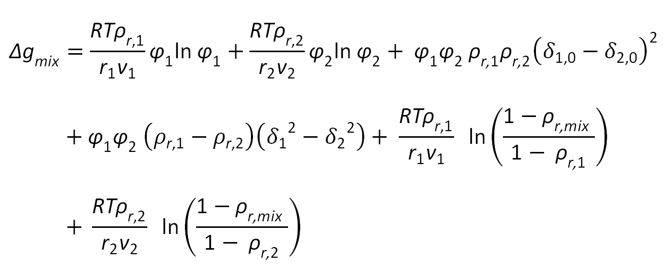
where ρ_r,i = ρ_i / ρ_i^* = v_i / v_hc,i is the reduced density which is simply a measure of the fractional occupied volume or, equivalently, one minus the fractional free volume in the compressible fluid, δ_0,i² = ρ_r,i δ_i² is the corresponding hardcore cohesive energy density, and φ₁ and φ₂ are the volume fractions of the two polymers,

φ_i = N_i r_i v_i / (N₁ r₁ v₁ + N₂ r₂ v₂) 

The first two terms of the Ruzette-Mayes equation are the classical combinatorial entropy of mixing and the third term is the classical exchange interaction energy of a regular solution, whereas the forth term arises from the very fact that the mixture is compressible, thus accounting for equation-of-state effects. The ffith and sixth terms describe the change in entropy due to expansion or contraction when mixing the two components. Mayes, Ruzette, and Gonzales-Leon neglected the last two terms as they are orders of magnitude smaller than the leading term. The model has been described in great detail by Ruzette and Gonzales.⁵ Below, we describe only how this model can be applied to polymer mixtures to calculate phase equilibria.

The Mayes-Ruzette equation for the free energy of mixing provides a simple explanation for the observed phase behavior of weakly interacting polymer systems. If for example (δ₁ - δ₂)² is (relative) large, like it is the case for polybutadiene-polystyrene (PBD-PS), it is the leading term and the blend shows only classical UCST behavior. However, the actual transition is only observable for rather low molecular weights or rather high temperatures, where the (small) entropy of mixing can dominate over the unfavorable interaction energy between unlike molecules.

However, when two polymers only weakly interact with each other (similar solubility parameters), the forth term becomes the leading energy term. At low temperatures, this term can become negative due to differences in the free volume of the pure components and cohensive energy density. This situation is often encountered when the polymer with the larger solubility parameter also has the larger free volume and larger thermal expansion coefficient (CTE). Since a negative free energy favors mixing, this polymer system does not show classical UCST behavior. However, with increasing temperature, the cohesive energy density of the component with the larger CTE will decrease faster than that of the other compound and at a certain point the forth term will become positive and, thus, the blend will become unstable, which means a LCST -type phase behavior is observed. In general, the phase behavior will depend on the relative magnitude of the mass densities, solubility parameters, and thermal expansion coefficients.

In part 2, it will be shown how phase diagrams for weakly interacting polymer blends can be predicted with Ruzette-Mayes Free Energy Model for compressible regular mixtures.

References & Notes

1. P. J. Flory, J. Chem. Phys. 9, 660 (1941); 10, 51 (1942)
2. M. L. Huggins, J. Phys. Chem. 46, 151 (1942); J. Am. Chem. Soc. 64, 1712 (1942)
3. Paul L. Flory, Principles of Polymer Chemistry, Ithaca, New york, 1953

4. The classical F-H model does not predict phase separation upon heating
   through the inverted miscibility gap (LCST), which is often observed for miscible or marginally miscible polymer mixtures and solutions.

5. Anne-Valerie G. Ruzette and Anne M. Mayes, Macromolecules 34, 1894-1907 (2001)

6. Juan A. Gonzalez-Leon and Anne M. Mayes, Macromolecules 36, 2508-2515 (2003)