Thermodynamic Equations of State of Polymers
Over the last 100 years, numerous P-V-T equations for liquids and gases have been developed. The relationships between volume (V), pressure (P) and temperature (T) are also called thermodynamic equations of state, or short equation of states (EOS). The simplest of these EOS is the ideal gas law:
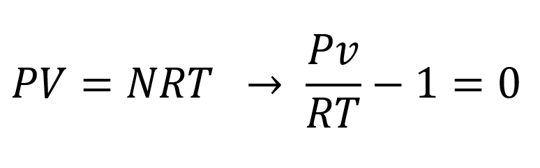
where N is the number of moles of substance, v is the molar volume, and R is the universal gas constant (R = 8.314 J/[mol·K]) which is the same for all fluids. The ideal gas equation assumes that the atoms and molecules are point particles (no specific volume) whose interactions with other particles are restricted to perfectly elastic impacts. The molecules of real gases, however, do have a specific volume which means that the accessible volume is less than the total volume of the system. The ideal gas equation also neglects the mutual attraction of the molecules caused by van der Waals and other forces. An equation that includes both effects is the so-called van der Waals equation:1
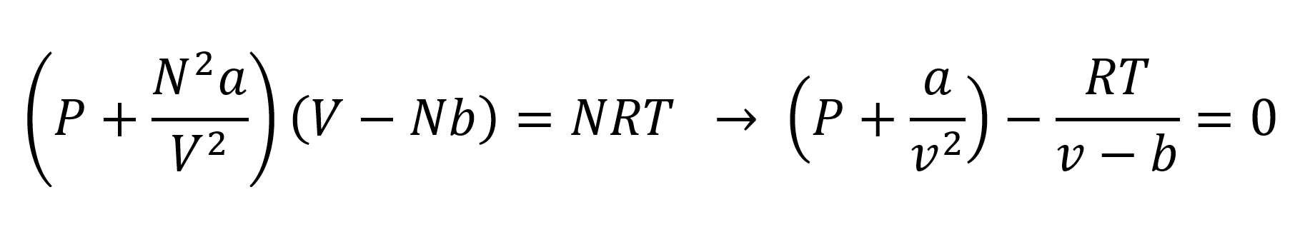
where a and b are the van der Waals correction factors for the reduced pressure and the reduced volume of the real gas molecules.
To simplify calculations, the equations of state are often written in terms of thermodynamic dimensionless parameters, that is as the ratio of the parameters to their value in the critical state (indicated by an asterisk):
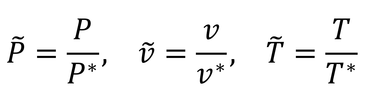
where the symbol ~ indicates reduced parameters. Introducing these quantities into the Van der Waals equation, we obtain an equation of state in dimensionless form which contains only universal constants (i.e. no material constants):
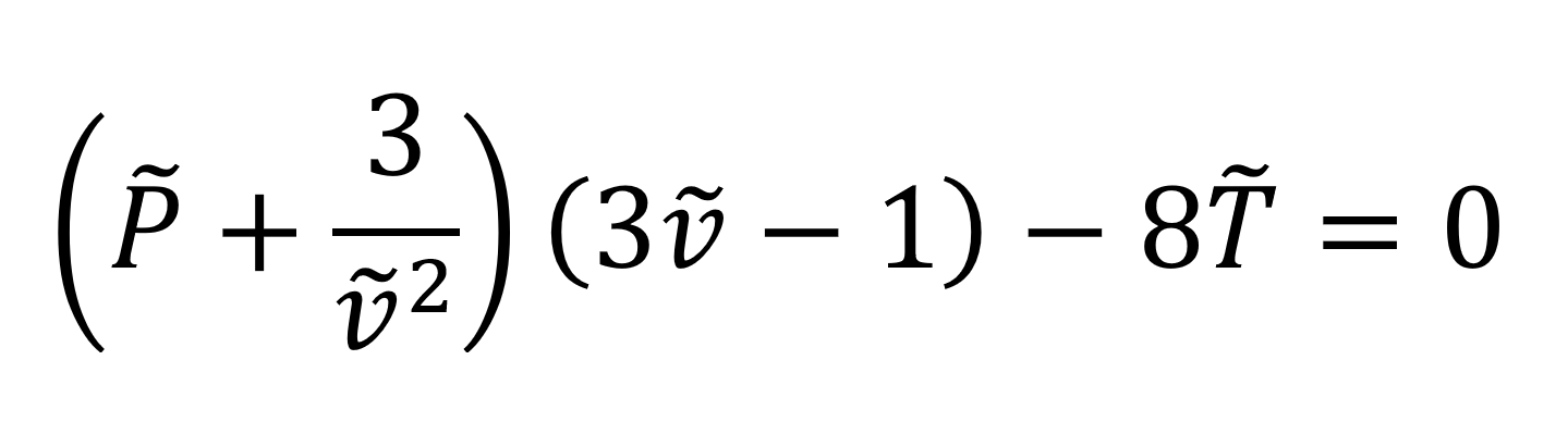
where we made use of the relations V* = 3b, P* =a/(27b2) and T* = (8/27) · (a/bR).2
The van der Waals equation is one of the simplest EOS and is often not accurate enough to describe the behavior of real fluids including liquid polymers. In general, any EOS can be written in the form
![]()
However, for more chemically complex liquids, a fourth parameter is usually needed to be able to accurately describe the relationship between T, P and V:3
![]()
This is the case for high molecular weight compounds such as amorphous polymers. The equations of state for these liquids can be broadly grouped into three types:4
- (Semi-)empirical PVT relations
- Cell models
- Lattice fluid models
Over the years, a large number of equations of state have been developed. Three of the most popular EOS frequently used for polymers are described below.
Tait's Empirical P-V-T Relation
One of the oldest purely empirical thermodynamic equation of state was developed by Peter Guthrie Tait in 1888.5 This equation reproduces the experimental liquid specific volumes (or liquid densities) over a wide pressure range. The most common form of the Tait equation is
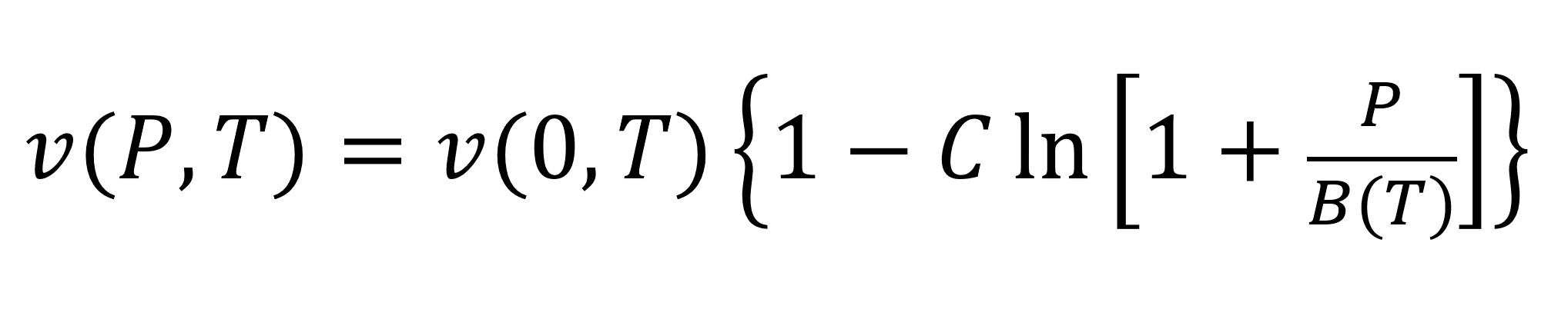
where C is a universal constant that has an average value of about 0.08946, v(0,T) is the specific volume at zero pressure, and B(T) is the Tait parameter for the liquid. The latter two parameters are a function only of temperature and are given by7
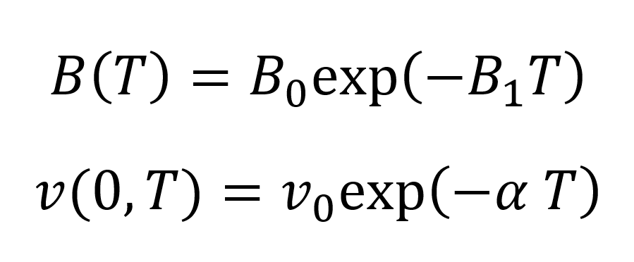
The parameter B0, B1 and v0 are specific constants for the polymer and α is the coefficient of volume expansion at zero pressure. These four constants can be obtained from P-V-T data and have been calculated for several common compounds.8
The Tait equation was originally developed to describe the compressibility of ordinary fluids. But as has been shown by Nanda and Simha (1964)9, it is also applicable to high molecular weight polymers in the real and hypothetical melt state, i.e. it is valid for polymers in the glassy state as well. In many cases, the maximum deviation between the calculated and experimental values is less than 2% and the average deviation is often within the reported experimental error.3,10
Sanchez-Lacombe Lattice Vacancy Model
One of the most popular theoretical equation of state (EOS) was developed by Sanchez and Lacombe in 1976.11 Their EOS is based on the lattice vacancy model which assumes random mixing of polymer chains and/or solvent molecules and holes (vacancies) on a lattice. Like in the Flory-Huggins model, each (macro)molecule is decomposed in a sequence of r segments (r-mers) that occupy r adjacent lattice cells. However, not all sites are occupied by polymer segments or solvent molecules, that is, some cells are empty (vacant). In other words, the density of the polymer melt or solution is allowed to vary by increasing or decreasing the volume fraction of vacancies in the lattice, whereas in the Flory-Huggins theory every site is occupied by either a polymer segment or solvent molecule.
The Sanchez and Lacombe model describes the liquid-vapor equilibrium
states of simple classical fluids reasonably
well below the critical point.11,13 also can be used to describe the
P-V-T behavior of polymers in the melt and amorphous solid state as well as the phase
equilibrium behavior of polymer mixtures and solutions.12
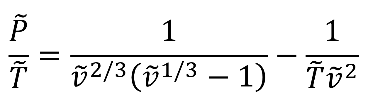
For the simple case of long polymer chains (r → ∞)
in the melt or amorphous state, the Sanchez-Lacombe EOS equation takes the
simple form12
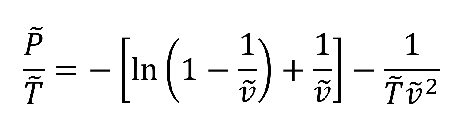
The temperature, pressure, and volume in the critical state can be calculated from11
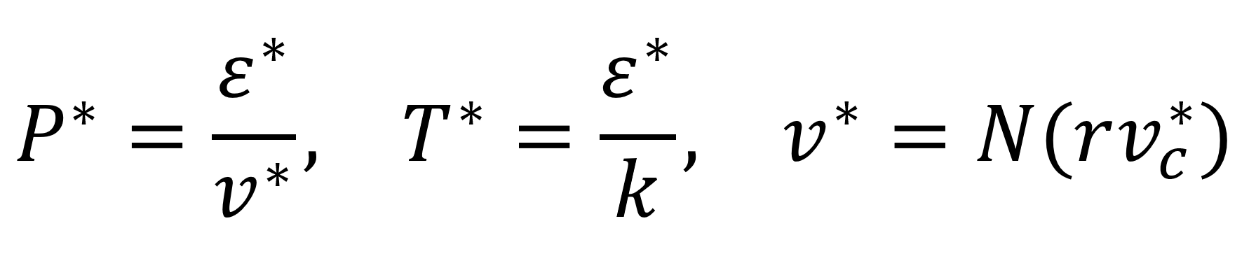
where ε* is the nonbonded interaction energy per mer, vc* is the close packed specific volume, and r is the number of segments per repeat unit. According to Sanchez and Lacombe, a pure fluid is completely characterized by these three molecular parameters (or by the three critical parameters P*, V*, and T*), which they tabulated for many classical fluids (solvents).11 They also calculated critical parameters for a number of common polymers by nonlinear least-squares fits of the above EOS to experimental liquid density data.12
Flory-Orwoll-Vrij Cell (OV) Model
One of the oldest theoretical equation of state for polymers in the melt and amorphous solid state was developed by Flory, Orwoll, and Vrij in 1964.14,15 Their model in reduced form has the simple mathematical form
Flory et al. derived their EOS specifically for liquid polymers. For this reason, it is not applicable to high temperatures and low densities (vapor phase). It also is less accurate than most (semi-empirical) EOS. Nonetheless, it still enjoys considerable popularity due to its simple mathematical form.
Theoretical Isotherms and Isobars for Polystyrene
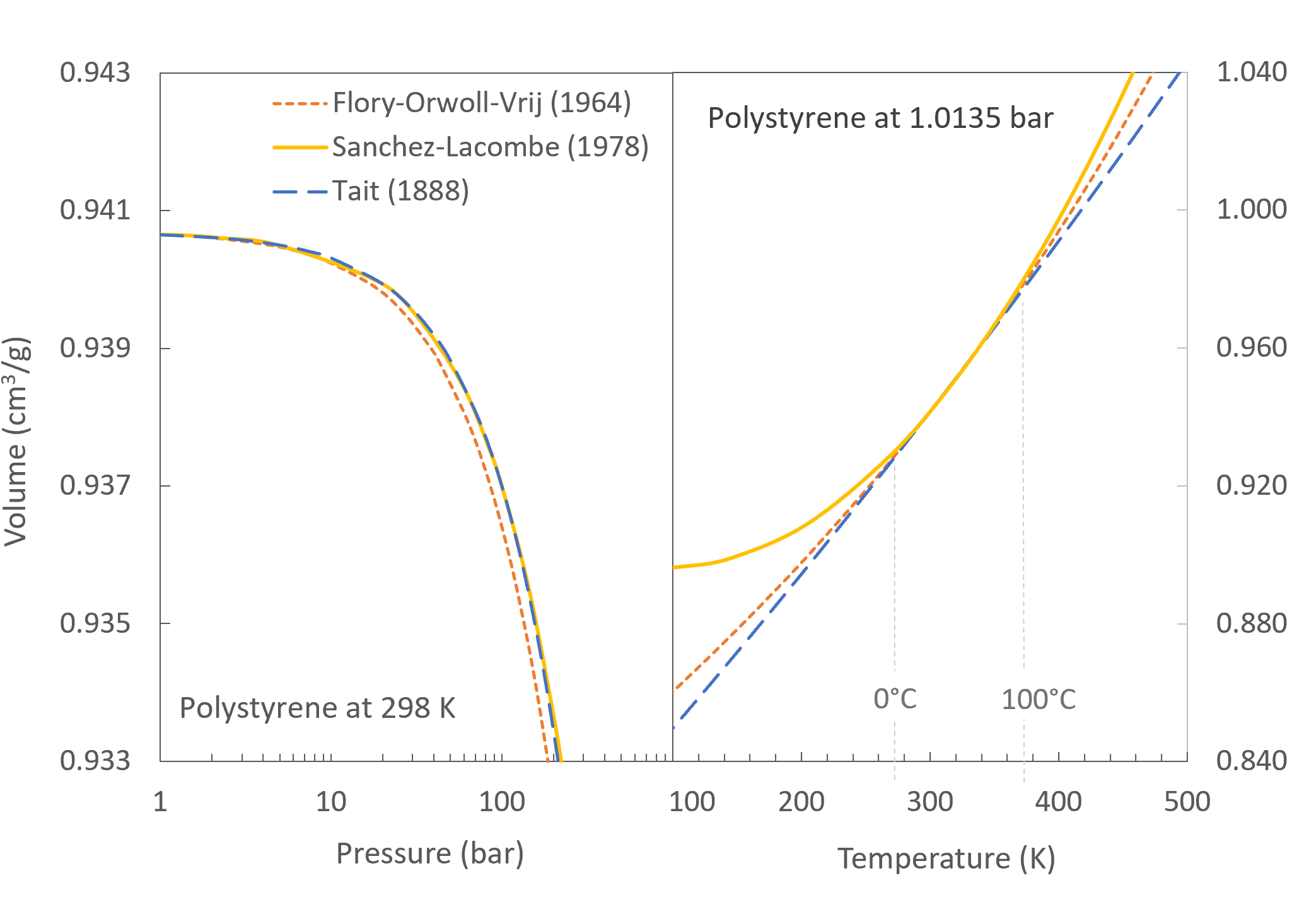
In the figures above, it can be seen that all three EOS equations give very similar isobars and isotherms when applied over a narrow pressure and temperature range, whereas for low and high temperatures the isotherms show some disagreement.16
References and Notes
Johannes Diderik van der Waals, Nobel Prize Lecture, The equation of state for gases
and liquids (1910)J.M. Prausnitz, R.N. Lichtenthal, E.G. de Azevedo, Molecular Thermodynamics of Fluid-
Phase Equilibria, Prentice-Hall Inc., New Jersey 1986- B. Kowalska, Int. Poly. Sci. & Technol., 29, 7 (2002)
- L.A. Utracki, C.A. Wilkie, Polymer Blends Handbook, Kluwer, Dordrecht 2003
- P. G. Tait, Phys. Chem., 2, 1 (1888)
- O. Olabisi, R. Simha, J. Appl. Poly. Sci., 21, 149-163 (1977)
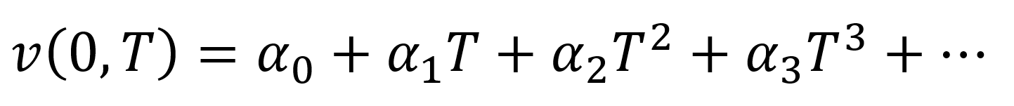
- The specific volume at zero (atmospheric) pressure, v(0,T), can also be fitted to a power series:
- R. Simha, P.S. Wilson, O. Olabisi, Kolloid-Z.u.Z.Polymere, 251, 6, 402-408 (1973)
- V.S. Nanda and R. Simha, J. Chem. Phys, 41, 1884 (1964)
R.P. Danner and M.S. High, Handbook of Polymer Solution Thermodynamics, American
Institute of Chemical Engineers, New York 1993- I. C. Sanchez and R. H. Lacombe, J. Phys. Chem., 80, 21, 2352 (1976)
- I. C. Sanchez and R. H. Lacombe, Macromolecules, 11, 6, 1145 (1978)
All mean-field theories break down near second-order phase transitions. Hence, the S-L theory does not yield accurate results near the critical point.
- P. J. Flory, R. A. Orwoll and A. Vrij, J. Am. Chem. Soc., 86. 3507 (1964)
- P. J. Flory, R. A. Orwoll and A. Vrij, J. Am. Chem. Soc., 86. 3515 (1964)
The isotherms and isobars have been calculated with the characteristic parameter of polystyrene listed in the Polymer Handbook by Brandup et al.17
J. Brandup, E.H. Immergut, and E.A. Grulke, Polymer Handbook, 4th Ed., VI / 591-601, Wiley, New York, 1999
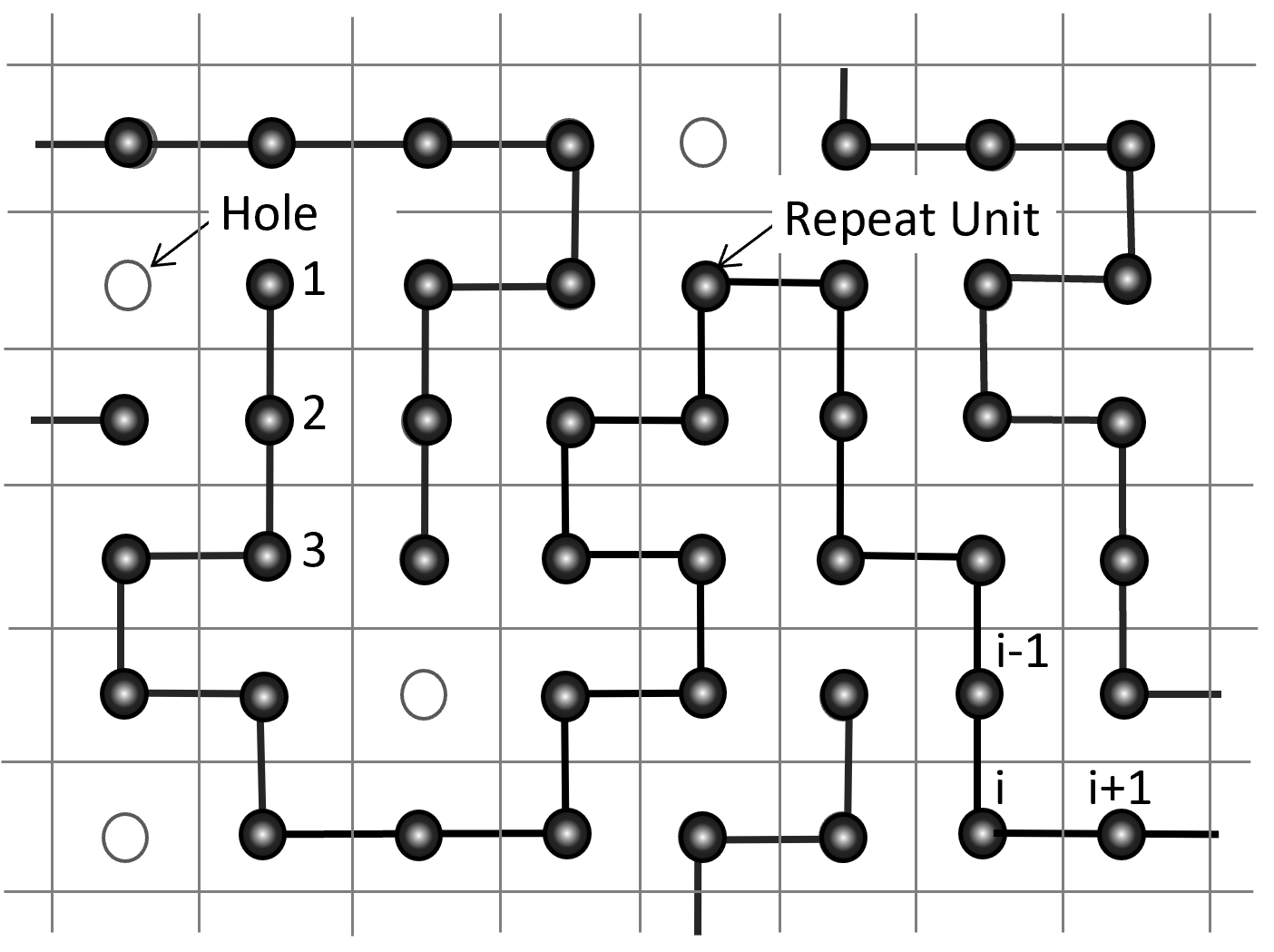 Two-dimensional pure lattice fluid with unoccupied sites (holes)