Polymers at Interfaces
Part2: Two-Order Parameter Mean-Field Theory

In the last 25 years numerous analytical self-consistent mean-field models were proposed to predict the structure of polymers near interfaces. One of the most elegant analytical mean-field models was developed by Semenov, Bonet-Avalos, Johner, and Joanny.¹ It describes the adsorption of homopolymers from good solvents (χ = 0) onto a flat homogenous surface. Their model goes beyond the standard ground state dominance approximation and not only predicts the total polymer volume fraction in the adsorbed layer φ_P(x) but also the contributions of loops φ_P^l(x), tails φ_P^t(x) and of free chains φ_P^fr(x) that penetrate the adsorbed layer. Below, their model will be applied to describe the polymer adsorption from a θ-solvent (χ = 1/2) which is of similar importance.

Semenov et al.^1-4 showed that the polymer concentration profile in the adsorbed layer near a homogenous interface can be described by two ground-state eigenfunctions g(x) and f(x):¹¹

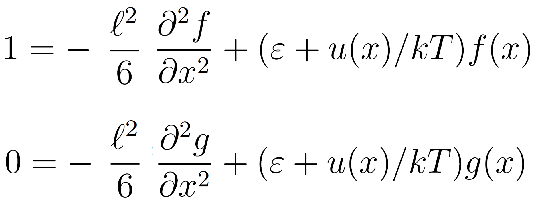
Because of the similarity of the two differential equations, f(x) can be computed from g(x):^2,6

Two partial integrations lead to^3,6,8

where

The equation above can be easily verified by differentiating it twice with respect to x and substituting the result into f g'' = g (f '' + 6/ ²).  

 

Concentration Profiles for Loops and Tails¹³

  

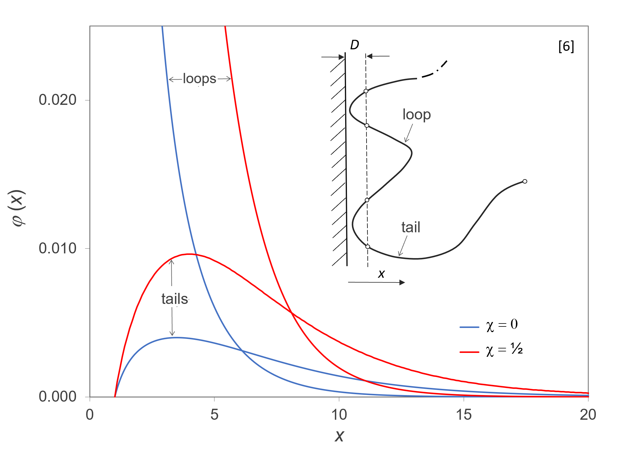
According to de Gennes and Semenov et al.^1,9, the adsorbed polymer layer, i.e. its concentration profile φ_P(x), can be divided into three distinct regions which de Gennes coined proximal, central and distal region. The monomer concentration in the region closest to the wall within a distance D (the so called proximal region) is directly affected by the surface-monomer interaction (χ_S), whereas in the intermediate or central region (D < x < d), the segment volume fraction φ_P(x) is dominated by short loops, and in the outer or distal region (x > d), tails are most abundant (φ_P^t >> φ_P^l).

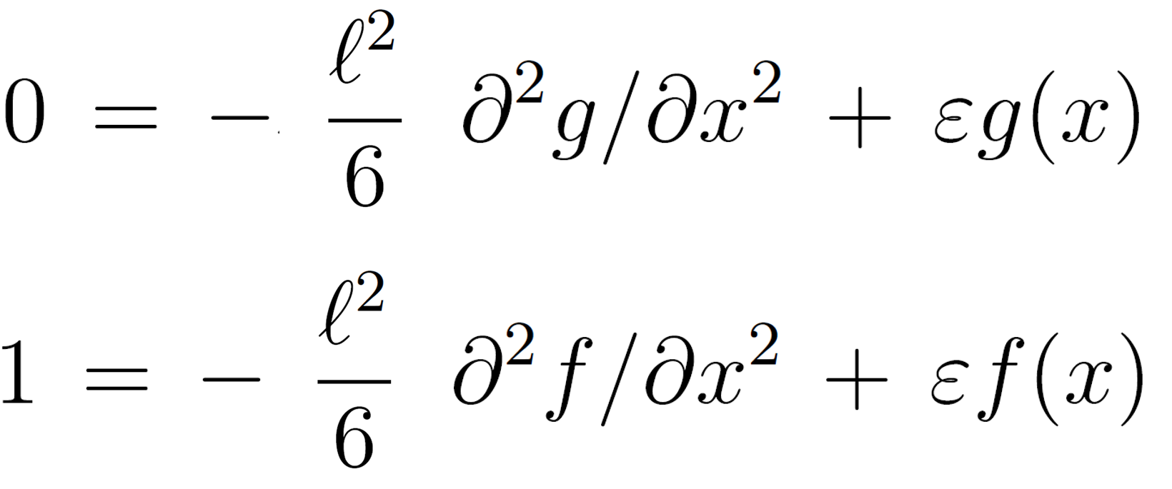
In a very dilute solution, the volume fraction of free polymers in the adsorbed layer can be neglected. For this case, the molecular potential u(x) simplifies to

Then the two order parameter equations for the central regime (D < x < ξ) with loop dominance can be written as

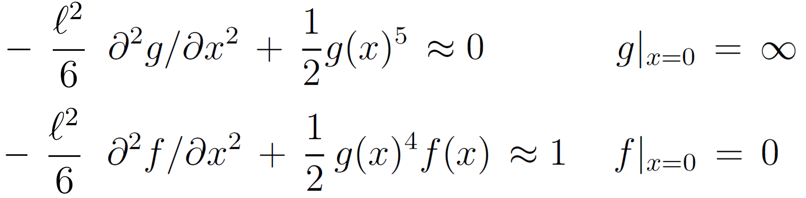
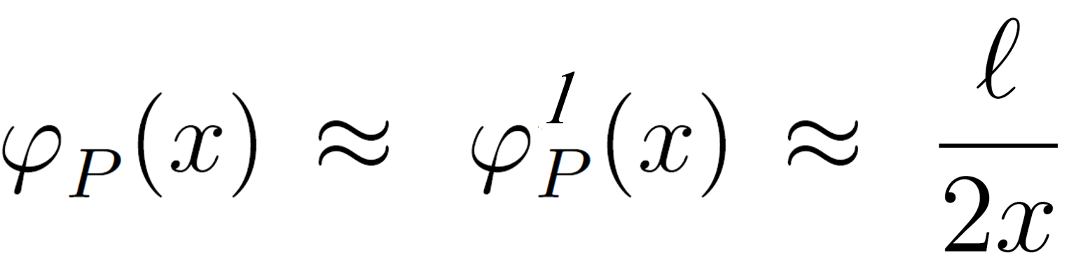
where we have assumed ε is negligible compared to u(x) which is only true for very long chains (N → ∞) and for the plateau regime where the polymer concentration is high and short loops dominate over tails, i.e. φ_P ≈ φ_P ^l ≈ g².^1,6 For this case, only the first differential equation needs to be solved which has the asymptotic solution

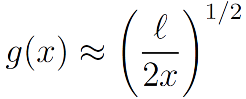
Then the polymer volume fraction in the loop dominated central regime reads

It is also possible that chain ends dominate. This is the case in the outer region of the central layer and for very weak adsorption where tails are much more abundant than loops. Assuming u(x) ≈ ½ φ_P^t(x) = ½ B g f, the two differential equations for the tail-dominated central regime read

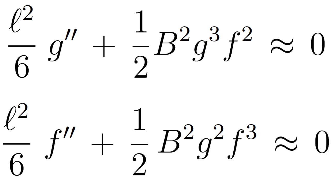
where B = 2b/N and b² = φ_P^∞e^εN. These two differential equations have the asymptotic solutions

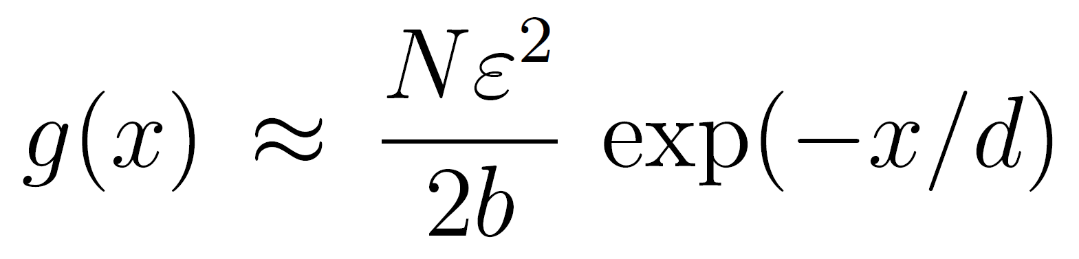
Then the polymer volume fraction in the tail dominated central regime reads

Comparing these results with those obtained by Semenov et al. for the athermal case (χ = 0),^4,12

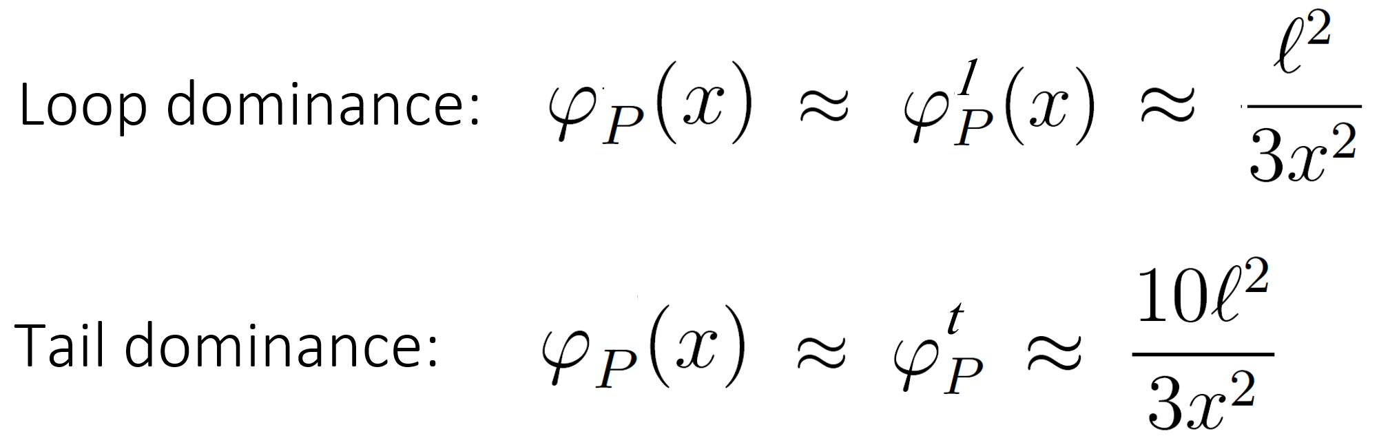
we find that the polymer concentration for χ = ½ decreases less rapidly with increasing distance to the surface (see figure above¹³).

The distal region (x > d) is mainly made up of tails; in this region, the polymer concentration is much lower than in the central region. Then the molecular potential u(x) is negligible compared to ε and the differential equations can be written in follwoing simplified form:

The first differential equation has the asymptotic solution⁴

The concentration of free chains is nearly constant and equal to bulk polymer volume fraction,φ_P^f ≈ φ_P^∞. Then the differential equation in f has the trivial solution f(x > d) ≈ 1 / ε. Since φ_P(x > d) ≈ φ_P^t(x) = 2b g f / N, the polymer volume fraction in the distal region has the simple solution⁴

Thus, the polymer concentration in the distal region decays exponentially, as predicted by de Gennes’ scaling theory.⁹

References and Notes

1. A.N. Semenov, J. Bonet-Avalos, A. Johner, J.F. Joanny, Macromolecules 29, 2179 (1996)

2. A. Johner, J.F. Joanny, M. Rubinstein, Europhys. Lett. 22, 591 (1993)

3. A.N. Semenov, J.F. Joanny, Europhys. Lett. 29, 279 (1995)

4. A. Johner, J. Bonet-Avalos, C.C. van der Linden, A.N. Semenov, J.F. Joanny, Macromolecules 29, 3629 (1996)

5. J. Bonet Avalos and A. Johner, Faraday Discuss. 98, 111-119 (1998)

6. G.J. Fleer, J. van Male, A. Johner, Macromolecules 32, 825 (1999) & 32, 845 (1999)

7. G.J. Fleer, F.A.M. Leermakers, Macromol. Symp. 126, 65 (1997)

8. M. Aubouy, E. Raphael, Macromolecules 27, 5182 (1994) u. 31, 4357 (1998)

9. P.G. de Gennes, Macromolecules 14, 1637-1644 (1981) & 15, 492-500 (1982)

10. G.J. Fleer, M.A. Cohen Stuart, J.M.H.M. Scheutjens, T. Cosgrove, B. Vincent; Polymers at Intefaces; Chapman & Hill, Cambridge (GB) 1993

11. It is assumed that the segment distribution is uniform in the y,z plane.

12. Semnove et al.^1,4 used reduced variables and normalized their results by the natural unit length
    ^* = 6^-1/2B^-1/3.

13. The curves depicted in the figure above have been calculated with the self-consistent mean-field theory proposed by Semenov et al.¹ and extended by Fleer et al.⁶ who proposed analytical solutions in closed form for both good solvents and θ-solvents. In this example, we chose χ_s = 1.0 and φ_p^∞=10^-6.